This page was generated from
docs/examples/transmission_ftir/PyIRoGlass_Transmission.ipynb.
Interactive online version:
![]() .
.
Transmission FTIR Spectra
This Jupyter notebook provides an example workflow for processing transmission FTIR spectra through PyIRoGlass.
The Jupyter notebook and data can be accessed here: https://github.com/SarahShi/PyIRoGlass/blob/main/docs/examples/transmission_ftir/.
You need to have the PyIRoGlass PyPi package on your machine once. If you have not done this, please uncomment (remove the #) symbol and run the cell below.
[1]:
#!pip install PyIRoGlass
Load Python Packages and Data
Load Python Packages
[2]:
# Import packages

import PyIRoGlass as pig

from IPython.display import Image

%matplotlib inline
%config InlineBackend.figure_format = 'retina'

pig.__version__
[2]:
'0.6.7'
Set paths to data
Update the path to the directory containing the spectra, as well as the paths to the chemistry and thickness data.
[3]:
spectrum_path = 'SPECTRA/'
print(spectrum_path)

chemistry_thickness_path = 'ChemThick.csv'
print(chemistry_thickness_path)
SPECTRA/
ChemThick.csv
Set desired output file directory name
Update the export_path to the desired output location.
[4]:
export_path = 'RESULTS'
print(export_path)
RESULTS
Load transmission FTIR spectra along with chemistry thickness data
We will use the class pig.SampleDataLoader to load all FTIR spectra and chemistry thickness data. The class takes the arguments:
spectrum_path: String or list path to the directory with spectral datachemistry_thickness_path: String path to CSV file with glass chemistry and thickness data
and contains the methods:
load_spectrum_directory: Loads spectral dataload_chemistry_thickness: Loads chemistry thickness dataload_all_data: Loads spectral and chemistry thickness data
Here, we use load_all_data. This returns the outputs of:
dfs_dict: Dictionary where the keys are file identifiers and values are DataFrames with spectral datachemistry: DataFrame of chemical datathickness: DataFrame of thickness data
The file names from the spectra (what comes before the .CSV) are important when we load in melt compositions and thicknesses. Unique identifiers identify the same samples. Make sure that this ChemThick.CSV file has the same sample names as the loaded spectra.
[5]:
loader = pig.SampleDataLoader(spectrum_path=spectrum_path, chemistry_thickness_path=chemistry_thickness_path)
dfs_dict, chemistry, thickness = loader.load_all_data()
Let’s look at what dfs_dict, a dictionary of transmission FTIR spectra, looks like. Samples are identified by their file names (keys) and the wavenumber and absorbance data are stored as dataframes for each spectrum (values).
[6]:
dfs_dict
[6]:
{'AC4_OL49_021920_30x30_H2O_a':             Absorbance
 Wavenumber
 1000.917      6.000000
 1002.845      6.000000
 1004.774      3.212358
 1006.702      6.000000
 1008.631      3.550053
 ...                ...
 5490.577      0.658218
 5492.505      0.657289
 5494.434      0.657169
 5496.362      0.658473
 5498.291      0.660256

 [2333 rows x 1 columns],
 'AC4_OL53_101220_256s_30x30_a':             Absorbance
 Wavenumber
 1000.916      6.000000
 1002.845      2.809911
 1004.774      2.584419
 1006.702      2.808356
 1008.631      3.712419
 ...                ...
 5490.576      0.118337
 5492.505      0.117460
 5494.433      0.117553
 5496.362      0.117506
 5498.291      0.116924

 [2333 rows x 1 columns],
 'STD_D1010_012821_256s_100x100_a':             Absorbance
 Wavenumber
 1000.916      3.844739
 1002.845      3.630789
 1004.774      6.000000
 1006.702      6.000000
 1008.631      6.000000
 ...                ...
 5490.576      0.394656
 5492.505      0.395436
 5494.433      0.396272
 5496.362      0.396495
 5498.291      0.396368

 [2333 rows x 1 columns]}
Display chemistry, the DataFrame of glass compositions.
[7]:
chemistry
[7]:
| SiO2 | TiO2 | Al2O3 | Fe2O3 | FeO | MnO | MgO | CaO | Na2O | K2O | P2O5 | |
|---|---|---|---|---|---|---|---|---|---|---|---|
| Sample | |||||||||||
| AC4_OL49_021920_30x30_H2O_a | 52.34 | 1.04 | 17.92 | 1.93 | 7.03 | 0.20 | 3.63 | 7.72 | 4.25 | 0.78 | 0.14 |
| AC4_OL53_101220_256s_30x30_a | 47.95 | 1.00 | 18.88 | 2.04 | 7.45 | 0.19 | 4.34 | 9.84 | 3.47 | 0.67 | 0.11 |
| STD_D1010_012821_256s_100x100_a | 51.41 | 1.26 | 16.58 | 0.00 | 7.58 | 0.00 | 7.57 | 10.98 | 3.01 | 0.37 | 0.18 |
Display thickness, the DataFrame of wafer thicknesses.
[8]:
thickness
[8]:
| Thickness | Sigma_Thickness | |
|---|---|---|
| Sample | ||
| AC4_OL49_021920_30x30_H2O_a | 91.25 | 3 |
| AC4_OL53_101220_256s_30x30_a | 39.00 | 3 |
| STD_D1010_012821_256s_100x100_a | 231.00 | 3 |
See that the sample names of the spectra in dfs_dict, chemistry, and thickness all align.
We’re ready to roll – MCMC, here we come!
We use the function pig.calculate_baselines, which takes in two arguments:
dfs_dict: Dictionary where the keys are file identifiers and values are DataFrames with spectral dataexport_path: Desired output directory name, orNoneto prevent figure generation
and returns:
Volatile_PH: DataFrame with peak heights and their associated uncertaintiesfailures: List of file identifiers for which analysis failed
Running this code will take a few seconds to minutes per spectra, as it is fitting \(\mathrm{10^6}\) baselines and peaks to your spectrum to sample uncertainty. If any samples fail, they will be returned in the list failures. It took 20 seconds to process 1 spectrum on my M2 Macbook Pro with 12 CPU cores. The same task takes about 2 minutes on Google Colab.
The function automatically saves this file as a CSV, so you have this information. We will also use this DataFrame to calculate concentrations.
[9]:
Volatile_PH, failures = pig.calculate_baselines(dfs_dict, export_path)
::::::::::::::::::::::::::::::::::::::::::::::::::::::::::::::::::::::
  Multi-core Markov-chain Monte Carlo (mc3).
  Version 3.2.1.
  Copyright (c) 2015-2026 Patricio Cubillos and collaborators.
  mc3 is open-source software under the MIT license (see LICENSE).
::::::::::::::::::::::::::::::::::::::::::::::::::::::::::::::::::::::


::::::::::::::::::::::::::::::::::::::::::::::::::::::::::::::::::::::
  Warning:
    The number of requested CPUs (4) is >= than the number of
available CPUs (2).  Enforced ncpu to 1.
::::::::::::::::::::::::::::::::::::::::::::::::::::::::::::::::::::::

Least-squares best-fitting parameters:
  [ 1.10352341e+00 -1.06147104e+00  9.35733625e-01 -9.21115401e-02
  3.00000000e-01  1.42788938e+03  2.88207409e+01  1.09418303e-01
  1.51745559e+03  3.58474224e+01  1.07059541e-01  6.59012777e-01
  1.22070954e-01  1.53688247e-02 -3.11486522e-04  1.23428193e+00]

Yippee Ki Yay Monte Carlo!
Start MCMC chains  (Wed Jul  8 19:04:46 2026)

[:         ]  10.0% completed  (Wed Jul  8 19:05:00 2026)
Out-of-bound Trials:
[   0    0    0    0 6565    0    0   20    0    0   42    0    0    0
    0    0]
Best Parameters: (chisq=369.0163)
[ 1.10352341e+00 -1.06147104e+00  9.35733625e-01 -9.21115401e-02
  3.00000000e-01  1.42788938e+03  2.88207409e+01  1.09418303e-01
  1.51745559e+03  3.58474224e+01  1.07059541e-01  6.59012777e-01
  1.22070954e-01  1.53688247e-02 -3.11486522e-04  1.23428193e+00]

[::        ]  20.0% completed  (Wed Jul  8 19:05:13 2026)
Out-of-bound Trials:
[    0    12     0     1 12941     0     2    21     0   893    44     0
     0     0     0     0]
Best Parameters: (chisq=369.0163)
[ 1.10352341e+00 -1.06147104e+00  9.35733625e-01 -9.21115401e-02
  3.00000000e-01  1.42788938e+03  2.88207409e+01  1.09418303e-01
  1.51745559e+03  3.58474224e+01  1.07059541e-01  6.59012777e-01
  1.22070954e-01  1.53688247e-02 -3.11486522e-04  1.23428193e+00]
Gelman-Rubin statistics for free parameters:
[1.05401139 1.05519132 1.01247758 1.05775097 1.04763765 1.08067766
 1.09390535 1.02282864 1.04398496 1.06344856 1.03324853 1.02129253
 1.02527753 1.03922281 1.05466767 1.05475236]

[:::       ]  30.0% completed  (Wed Jul  8 19:05:26 2026)
Out-of-bound Trials:
[    0    54     0    13 23569     0    30    23     0  3987    48     0
     0     0     0     0]
Best Parameters: (chisq=369.0163)
[ 1.10352341e+00 -1.06147104e+00  9.35733625e-01 -9.21115401e-02
  3.00000000e-01  1.42788938e+03  2.88207409e+01  1.09418303e-01
  1.51745559e+03  3.58474224e+01  1.07059541e-01  6.59012777e-01
  1.22070954e-01  1.53688247e-02 -3.11486522e-04  1.23428193e+00]
Gelman-Rubin statistics for free parameters:
[1.00814651 1.00949798 1.00138293 1.01037902 1.00301833 1.01369397
 1.01223094 1.00526289 1.00333309 1.01220576 1.00548864 1.00154711
 1.0022855  1.00694136 1.00890332 1.00980786]

[::::      ]  40.0% completed  (Wed Jul  8 19:05:39 2026)
Out-of-bound Trials:
[    0   129     0    32 35847     1    69    25     1  7703    54     0
     0     0     0     0]
Best Parameters: (chisq=369.0163)
[ 1.10352341e+00 -1.06147104e+00  9.35733625e-01 -9.21115401e-02
  3.00000000e-01  1.42788938e+03  2.88207409e+01  1.09418303e-01
  1.51745559e+03  3.58474224e+01  1.07059541e-01  6.59012777e-01
  1.22070954e-01  1.53688247e-02 -3.11486522e-04  1.23428193e+00]
Gelman-Rubin statistics for free parameters:
[1.00134307 1.00173038 1.00048907 1.00195797 1.00101743 1.00529828
 1.00381316 1.00139341 1.00117366 1.0038627  1.00263982 1.00056887
 1.00166879 1.00304886 1.00158981 1.00182516]
All parameters converged to within 1% of unity.

[:::::     ]  50.0% completed  (Wed Jul  8 19:05:52 2026)
Out-of-bound Trials:
[    0   235     0    42 48612     2   119    27     1 11396    56     0
     0     0     0     0]
Best Parameters: (chisq=369.0163)
[ 1.10352341e+00 -1.06147104e+00  9.35733625e-01 -9.21115401e-02
  3.00000000e-01  1.42788938e+03  2.88207409e+01  1.09418303e-01
  1.51745559e+03  3.58474224e+01  1.07059541e-01  6.59012777e-01
  1.22070954e-01  1.53688247e-02 -3.11486522e-04  1.23428193e+00]
Gelman-Rubin statistics for free parameters:
[1.00070269 1.00078841 1.00074722 1.00101368 1.00042546 1.00239575
 1.00177335 1.00063257 1.00098102 1.00177017 1.00178554 1.0012747
 1.00108406 1.001285   1.00077068 1.00081165]
All parameters converged to within 1% of unity.

[::::::    ]  60.0% completed  (Wed Jul  8 19:06:04 2026)
Out-of-bound Trials:
[    0   342     0    56 61095     3   175    28     1 15504    60     0
     0     0     0     0]
Best Parameters: (chisq=369.0163)
[ 1.10352341e+00 -1.06147104e+00  9.35733625e-01 -9.21115401e-02
  3.00000000e-01  1.42788938e+03  2.88207409e+01  1.09418303e-01
  1.51745559e+03  3.58474224e+01  1.07059541e-01  6.59012777e-01
  1.22070954e-01  1.53688247e-02 -3.11486522e-04  1.23428193e+00]
Gelman-Rubin statistics for free parameters:
[1.00087322 1.00099674 1.00028822 1.00099221 1.00042128 1.00113043
 1.00147478 1.0005011  1.000913   1.00105709 1.00079193 1.00094712
 1.00072302 1.00067012 1.00101069 1.00105984]
All parameters converged to within 1% of unity.

All parameters satisfy the GR convergence threshold of 1.01, stopping
the MCMC.

MCMC Summary:
-------------
  Number of evaluated samples:        601335
  Number of parallel chains:               9
  Average iterations per chain:        66815
  Burned-in iterations per chain:      20000
  Thinning factor:                         5
  MCMC sample size (thinned, burned):  84267
  Acceptance rate:   24.55%

Parameter name     best fit   median      1sigma_low   1sigma_hi        S/N
--------------- -----------  -----------------------------------  ---------
B_mean           1.1035e+00   1.1306e+00 -3.3185e-02  4.1162e-02       28.8
B_PC1           -1.0615e+00  -7.8199e-01 -3.5748e-01  4.2742e-01        2.6
B_PC2            9.3573e-01   9.3269e-01 -1.9815e-02  2.0363e-02       46.8
B_PC3           -9.2112e-02  -5.7634e-02 -5.7032e-02  6.2859e-02        1.5
B_PC4            3.0000e-01   2.7972e-01 -3.0201e-02  1.5061e-02       12.4
G1430_peak       1.4279e+03   1.4279e+03 -1.3717e+00  1.5053e+00      998.4
G1430_std        2.8821e+01   2.8799e+01 -1.1719e+00  1.2321e+00       24.0
G1430_amp        1.0942e-01   1.0869e-01 -4.0989e-03  4.0358e-03       26.8
G1515_peak       1.5175e+03   1.5176e+03 -1.5380e+00  1.5079e+00      984.7
G1515_std        3.5847e+01   3.6110e+01 -2.1569e+00  2.1048e+00       17.9
G1515_amp        1.0706e-01   1.0696e-01 -3.6161e-03  3.6743e-03       29.6
H1635_mean       6.5901e-01   6.5931e-01 -3.1508e-03  3.1455e-03      212.0
H1635_PC1        1.2207e-01   1.2008e-01 -1.4374e-02  1.4514e-02        8.5
H1635_PC2        1.5369e-02   1.4715e-02 -2.2538e-02  2.1779e-02        0.7
m               -3.1149e-04  -2.6407e-04 -6.0463e-05  7.2956e-05        4.5
b                1.2343e+00   1.2202e+00 -2.2633e-02  1.9200e-02       57.1

  Best-parameter's chi-squared:       367.5930
  Best-parameter's -2*log(posterior): 369.0163
  Bayesian Information Criterion:     469.8369
  Reduced chi-squared:                  0.6338
  Standard deviation of residuals:  0.00785345

For a detailed summary with all parameter posterior statistics see
/home/docs/checkouts/readthedocs.org/user_builds/pyiroglass/checkouts/latest/docs/examples/transmission_ftir/NPZTXTFILES/RESULTS/AC4_OL49_021920_30x30_H2O_a_statistics.txt

Output sampler files:
  /home/docs/checkouts/readthedocs.org/user_builds/pyiroglass/checkouts/latest/docs/examples/transmission_ftir/NPZTXTFILES/RESULTS/AC4_OL49_021920_30x30_H2O_a_statistics.txt
  /home/docs/checkouts/readthedocs.org/user_builds/pyiroglass/checkouts/latest/docs/examples/transmission_ftir/NPZTXTFILES/RESULTS/AC4_OL49_021920_30x30_H2O_a.npz
  /home/docs/checkouts/readthedocs.org/user_builds/pyiroglass/checkouts/latest/docs/examples/transmission_ftir/LOGFILES/RESULTS/AC4_OL49_021920_30x30_H2O_a.log

::::::::::::::::::::::::::::::::::::::::::::::::::::::::::::::::::::::
  Multi-core Markov-chain Monte Carlo (mc3).
  Version 3.2.1.
  Copyright (c) 2015-2026 Patricio Cubillos and collaborators.
  mc3 is open-source software under the MIT license (see LICENSE).
::::::::::::::::::::::::::::::::::::::::::::::::::::::::::::::::::::::


::::::::::::::::::::::::::::::::::::::::::::::::::::::::::::::::::::::
  Warning:
    The number of requested CPUs (4) is >= than the number of
available CPUs (2).  Enforced ncpu to 1.
::::::::::::::::::::::::::::::::::::::::::::::::::::::::::::::::::::::

Least-squares best-fitting parameters:
  [ 5.11148189e-01 -2.96910196e+00  2.75566352e-01 -5.06622408e-01
  2.27844162e-01  1.42739189e+03  3.45255612e+01  5.04958691e-02
  1.51924154e+03  3.21665127e+01  5.31133455e-02  3.00626999e-01
 -3.90990542e-02  5.29060293e-02 -4.45749758e-04  7.21455954e-01]

Yippee Ki Yay Monte Carlo!
Start MCMC chains  (Wed Jul  8 19:06:19 2026)

[:         ]  10.0% completed  (Wed Jul  8 19:06:32 2026)
Out-of-bound Trials:
[   0 7934    0  242  559   43 1327  238   25  231  245    1    0    0
    0    0]
Best Parameters: (chisq=49.0306)
[ 5.11148189e-01 -2.96910196e+00  2.75566352e-01 -5.06622408e-01
  2.27844162e-01  1.42739189e+03  3.45255612e+01  5.04958691e-02
  1.51924154e+03  3.21665127e+01  5.31133455e-02  3.00626999e-01
 -3.90990542e-02  5.29060293e-02 -4.45749758e-04  7.21455954e-01]

[::        ]  20.0% completed  (Wed Jul  8 19:06:45 2026)
Out-of-bound Trials:
[    1 17840     0   738  1455   186  4182   286    82  1378   289     1
     0     0     0     0]
Best Parameters: (chisq=49.0306)
[ 5.11148189e-01 -2.96910196e+00  2.75566352e-01 -5.06622408e-01
  2.27844162e-01  1.42739189e+03  3.45255612e+01  5.04958691e-02
  1.51924154e+03  3.21665127e+01  5.31133455e-02  3.00626999e-01
 -3.90990542e-02  5.29060293e-02 -4.45749758e-04  7.21455954e-01]
Gelman-Rubin statistics for free parameters:
[1.02493194 1.02418202 1.01433947 1.02673464 1.0111879  1.0368794
 1.02398951 1.00412487 1.03168607 1.05712374 1.00426059 1.01103396
 1.01370669 1.00920284 1.02508482 1.02510585]

[:::       ]  30.0% completed  (Wed Jul  8 19:06:58 2026)
Out-of-bound Trials:
[    2 27099     0  1388  2462   387  8264   311   136  3074   309     1
     0     0     0     0]
Best Parameters: (chisq=49.0306)
[ 5.11148189e-01 -2.96910196e+00  2.75566352e-01 -5.06622408e-01
  2.27844162e-01  1.42739189e+03  3.45255612e+01  5.04958691e-02
  1.51924154e+03  3.21665127e+01  5.31133455e-02  3.00626999e-01
 -3.90990542e-02  5.29060293e-02 -4.45749758e-04  7.21455954e-01]
Gelman-Rubin statistics for free parameters:
[1.00671141 1.00732877 1.00102558 1.00754518 1.00378353 1.00693856
 1.00184809 1.00178668 1.00159444 1.00936194 1.00242394 1.00186388
 1.00422078 1.00777771 1.00723667 1.00776678]
All parameters converged to within 1% of unity.

[::::      ]  40.0% completed  (Wed Jul  8 19:07:11 2026)
Out-of-bound Trials:
[    9 37217     0  2090  3587   609 12510   348   197  5136   331     1
     0     0     0     0]
Best Parameters: (chisq=49.0306)
[ 5.11148189e-01 -2.96910196e+00  2.75566352e-01 -5.06622408e-01
  2.27844162e-01  1.42739189e+03  3.45255612e+01  5.04958691e-02
  1.51924154e+03  3.21665127e+01  5.31133455e-02  3.00626999e-01
 -3.90990542e-02  5.29060293e-02 -4.45749758e-04  7.21455954e-01]
Gelman-Rubin statistics for free parameters:
[1.00303304 1.00313395 1.00236921 1.0025383  1.00322597 1.00570971
 1.00146825 1.00202883 1.00171575 1.00644094 1.00150032 1.00122545
 1.00289907 1.00452509 1.00300227 1.00297484]
All parameters converged to within 1% of unity.

[:::::     ]  50.0% completed  (Wed Jul  8 19:07:24 2026)
Out-of-bound Trials:
[   15 47993     0  2855  4727   835 16672   359   241  7106   351     1
     0     0     0     0]
Best Parameters: (chisq=49.0306)
[ 5.11148189e-01 -2.96910196e+00  2.75566352e-01 -5.06622408e-01
  2.27844162e-01  1.42739189e+03  3.45255612e+01  5.04958691e-02
  1.51924154e+03  3.21665127e+01  5.31133455e-02  3.00626999e-01
 -3.90990542e-02  5.29060293e-02 -4.45749758e-04  7.21455954e-01]
Gelman-Rubin statistics for free parameters:
[1.00121954 1.00132883 1.0011362  1.00094447 1.00175093 1.00278997
 1.00115373 1.00103102 1.00107723 1.0029356  1.0008687  1.00056631
 1.00121717 1.00199931 1.00121202 1.00122668]
All parameters converged to within 1% of unity.

[::::::    ]  60.0% completed  (Wed Jul  8 19:07:37 2026)
Out-of-bound Trials:
[   21 58015     0  3632  5923  1086 20908   375   296  9222   359     1
     0     0     0     0]
Best Parameters: (chisq=49.0306)
[ 5.11148189e-01 -2.96910196e+00  2.75566352e-01 -5.06622408e-01
  2.27844162e-01  1.42739189e+03  3.45255612e+01  5.04958691e-02
  1.51924154e+03  3.21665127e+01  5.31133455e-02  3.00626999e-01
 -3.90990542e-02  5.29060293e-02 -4.45749758e-04  7.21455954e-01]
Gelman-Rubin statistics for free parameters:
[1.00074465 1.00063795 1.00101622 1.00050912 1.00124075 1.00151717
 1.00097704 1.00066309 1.00082192 1.00205715 1.00083714 1.00043596
 1.00117639 1.00130412 1.0006478  1.00056373]
All parameters converged to within 1% of unity.

All parameters satisfy the GR convergence threshold of 1.01, stopping
the MCMC.

MCMC Summary:
-------------
  Number of evaluated samples:        601605
  Number of parallel chains:               9
  Average iterations per chain:        66845
  Burned-in iterations per chain:      20000
  Thinning factor:                         5
  MCMC sample size (thinned, burned):  84321
  Acceptance rate:   22.01%

Parameter name     best fit   median      1sigma_low   1sigma_hi        S/N
--------------- -----------  -----------------------------------  ---------
B_mean           5.1115e-01   5.5725e-01 -3.4643e-02  5.3873e-02       11.4
B_PC1           -2.9691e+00  -2.4897e+00 -3.5675e-01  5.6017e-01        6.5
B_PC2            2.7557e-01   2.7022e-01 -2.0522e-02  2.0517e-02       13.4
B_PC3           -5.0662e-01  -4.4545e-01 -5.0268e-02  7.2395e-02        8.1
B_PC4            2.2784e-01   1.8882e-01 -4.5905e-02  3.8909e-02        5.3
G1430_peak       1.4274e+03   1.4272e+03 -3.1572e+00  3.1020e+00      460.1
G1430_std        3.4526e+01   3.4576e+01 -2.9239e+00  2.8740e+00       12.6
G1430_amp        5.0496e-02   5.0059e-02 -4.2831e-03  4.4523e-03       11.6
G1515_peak       1.5192e+03   1.5195e+03 -2.7564e+00  2.7595e+00      547.5
G1515_std        3.2167e+01   3.2859e+01 -2.6495e+00  3.0128e+00       11.7
G1515_amp        5.3113e-02   5.3359e-02 -3.7230e-03  3.8888e-03       14.2
H1635_mean       3.0063e-01   3.0112e-01 -3.1078e-03  3.0822e-03       96.8
H1635_PC1       -3.9099e-02  -4.1278e-02 -1.4686e-02  1.4307e-02        2.7
H1635_PC2        5.2906e-02   5.2215e-02 -1.9055e-02  1.7940e-02        2.8
m               -4.4575e-04  -3.6429e-04 -6.0936e-05  9.4946e-05        5.7
b                7.2146e-01   6.9688e-01 -2.8688e-02  1.8510e-02       30.6

  Best-parameter's chi-squared:        48.0236
  Best-parameter's -2*log(posterior):  49.0306
  Bayesian Information Criterion:     150.2674
  Reduced chi-squared:                  0.0828
  Standard deviation of residuals:  0.0028386

For a detailed summary with all parameter posterior statistics see
/home/docs/checkouts/readthedocs.org/user_builds/pyiroglass/checkouts/latest/docs/examples/transmission_ftir/NPZTXTFILES/RESULTS/AC4_OL53_101220_256s_30x30_a_statistics.txt

Output sampler files:
  /home/docs/checkouts/readthedocs.org/user_builds/pyiroglass/checkouts/latest/docs/examples/transmission_ftir/NPZTXTFILES/RESULTS/AC4_OL53_101220_256s_30x30_a_statistics.txt
  /home/docs/checkouts/readthedocs.org/user_builds/pyiroglass/checkouts/latest/docs/examples/transmission_ftir/NPZTXTFILES/RESULTS/AC4_OL53_101220_256s_30x30_a.npz
  /home/docs/checkouts/readthedocs.org/user_builds/pyiroglass/checkouts/latest/docs/examples/transmission_ftir/LOGFILES/RESULTS/AC4_OL53_101220_256s_30x30_a.log

::::::::::::::::::::::::::::::::::::::::::::::::::::::::::::::::::::::
  Multi-core Markov-chain Monte Carlo (mc3).
  Version 3.2.1.
  Copyright (c) 2015-2026 Patricio Cubillos and collaborators.
  mc3 is open-source software under the MIT license (see LICENSE).
::::::::::::::::::::::::::::::::::::::::::::::::::::::::::::::::::::::


::::::::::::::::::::::::::::::::::::::::::::::::::::::::::::::::::::::
  Warning:
    The number of requested CPUs (4) is >= than the number of
available CPUs (2).  Enforced ncpu to 1.
::::::::::::::::::::::::::::::::::::::::::::::::::::::::::::::::::::::

Least-squares best-fitting parameters:
  [ 4.00000000e+00  7.53559841e-01 -4.45578621e-01 -3.77207820e-01
  1.77129448e-01  1.43150803e+03  3.10778810e+01  6.77796837e-02
  1.52279968e+03  3.51836389e+01  7.59276789e-02  1.73134549e-01
  6.68571581e-02 -3.77536829e-02 -2.32934277e-04  2.46271034e+00]

Yippee Ki Yay Monte Carlo!
Start MCMC chains  (Wed Jul  8 19:07:51 2026)

[:         ]  10.0% completed  (Wed Jul  8 19:08:04 2026)
Out-of-bound Trials:
[19870     0     0    65   137    33    19    60    20   210    83     6
     0     1     0     0]
Best Parameters: (chisq=1775.0923)
[ 4.00000000e+00  7.53559841e-01 -4.45578621e-01 -3.77207820e-01
  1.77129448e-01  1.43150803e+03  3.10778810e+01  6.77796837e-02
  1.52279968e+03  3.51836389e+01  7.59276789e-02  1.73134549e-01
  6.68571581e-02 -3.77536829e-02 -2.32934277e-04  2.46271034e+00]

[::        ]  20.0% completed  (Wed Jul  8 19:08:16 2026)
Out-of-bound Trials:
[36802     4     0   165   359   105   199    81    72  1952   102     7
     0     1     0     0]
Best Parameters: (chisq=1775.0923)
[ 4.00000000e+00  7.53559841e-01 -4.45578621e-01 -3.77207820e-01
  1.77129448e-01  1.43150803e+03  3.10778810e+01  6.77796837e-02
  1.52279968e+03  3.51836389e+01  7.59276789e-02  1.73134549e-01
  6.68571581e-02 -3.77536829e-02 -2.32934277e-04  2.46271034e+00]
Gelman-Rubin statistics for free parameters:
[1.02209093 1.00737908 1.01218101 1.02792832 1.06523439 1.02985687
 1.14558422 1.01604572 1.04782088 1.02706834 1.02911711 1.01463572
 1.00575236 1.02105744 1.02154043 1.02156169]

[:::       ]  30.0% completed  (Wed Jul  8 19:08:29 2026)
Out-of-bound Trials:
[53169     4     0   226   496   149   534    98   145  6327   109     8
     0     1     0     0]
Best Parameters: (chisq=1775.0923)
[ 4.00000000e+00  7.53559841e-01 -4.45578621e-01 -3.77207820e-01
  1.77129448e-01  1.43150803e+03  3.10778810e+01  6.77796837e-02
  1.52279968e+03  3.51836389e+01  7.59276789e-02  1.73134549e-01
  6.68571581e-02 -3.77536829e-02 -2.32934277e-04  2.46271034e+00]
Gelman-Rubin statistics for free parameters:
[1.00413821 1.00300524 1.0032606  1.00286201 1.0015885  1.00210965
 1.00415564 1.00251234 1.00199937 1.00541905 1.00167708 1.00207368
 1.00258356 1.00390251 1.00392265 1.00336552]
All parameters converged to within 1% of unity.

[::::      ]  40.0% completed  (Wed Jul  8 19:08:41 2026)
Out-of-bound Trials:
[68870     5     0   279   683   199  1113   104   227 10925   118     8
     0     1     0     0]
Best Parameters: (chisq=1775.0923)
[ 4.00000000e+00  7.53559841e-01 -4.45578621e-01 -3.77207820e-01
  1.77129448e-01  1.43150803e+03  3.10778810e+01  6.77796837e-02
  1.52279968e+03  3.51836389e+01  7.59276789e-02  1.73134549e-01
  6.68571581e-02 -3.77536829e-02 -2.32934277e-04  2.46271034e+00]
Gelman-Rubin statistics for free parameters:
[1.00250238 1.00136606 1.00089095 1.0010583  1.00082747 1.00108489
 1.00148111 1.00130257 1.00095115 1.00288294 1.0003375  1.00118156
 1.00085211 1.00254259 1.00191036 1.00124183]
All parameters converged to within 1% of unity.

[:::::     ]  50.0% completed  (Wed Jul  8 19:08:54 2026)
Out-of-bound Trials:
[84430     9     0   324   868   259  1717   108   321 15706   124     8
     0     1     0     0]
Best Parameters: (chisq=1775.0923)
[ 4.00000000e+00  7.53559841e-01 -4.45578621e-01 -3.77207820e-01
  1.77129448e-01  1.43150803e+03  3.10778810e+01  6.77796837e-02
  1.52279968e+03  3.51836389e+01  7.59276789e-02  1.73134549e-01
  6.68571581e-02 -3.77536829e-02 -2.32934277e-04  2.46271034e+00]
Gelman-Rubin statistics for free parameters:
[1.00136316 1.00093045 1.00051054 1.00059271 1.00085189 1.00070834
 1.00147023 1.00039626 1.00100121 1.00155887 1.00100508 1.00175718
 1.00045125 1.00174438 1.00118425 1.00087521]
All parameters converged to within 1% of unity.

[::::::    ]  60.0% completed  (Wed Jul  8 19:09:06 2026)
Out-of-bound Trials:
[99547    11     0   385  1060   337  2399   114   450 20458   128     8
     0     1     0     0]
Best Parameters: (chisq=1775.0923)
[ 4.00000000e+00  7.53559841e-01 -4.45578621e-01 -3.77207820e-01
  1.77129448e-01  1.43150803e+03  3.10778810e+01  6.77796837e-02
  1.52279968e+03  3.51836389e+01  7.59276789e-02  1.73134549e-01
  6.68571581e-02 -3.77536829e-02 -2.32934277e-04  2.46271034e+00]
Gelman-Rubin statistics for free parameters:
[1.00133966 1.00096086 1.00058333 1.0007257  1.00031285 1.00038949
 1.00068654 1.00022399 1.00062504 1.00142635 1.00046495 1.00091015
 1.00049555 1.00138414 1.00127101 1.00095413]
All parameters converged to within 1% of unity.

All parameters satisfy the GR convergence threshold of 1.01, stopping
the MCMC.

MCMC Summary:
-------------
  Number of evaluated samples:        601300
  Number of parallel chains:               9
  Average iterations per chain:        66811
  Burned-in iterations per chain:      20000
  Thinning factor:                         5
  MCMC sample size (thinned, burned):  84260
  Acceptance rate:   20.86%

Parameter name     best fit   median      1sigma_low   1sigma_hi        S/N
--------------- -----------  -----------------------------------  ---------
B_mean           4.0000e+00   3.9956e+00 -6.9420e-03  3.2879e-03      679.8
B_PC1            7.5356e-01   6.9419e-01 -9.8409e-02  9.2160e-02        7.7
B_PC2           -4.4558e-01  -4.4469e-01 -1.9363e-02  1.8940e-02       23.3
B_PC3           -3.7721e-01  -3.8616e-01 -2.6801e-02  2.6518e-02       14.2
B_PC4            1.7713e-01   1.8310e-01 -2.2933e-02  2.4478e-02        7.4
G1430_peak       1.4315e+03   1.4317e+03 -2.2102e+00  2.3938e+00      621.0
G1430_std        3.1078e+01   3.1491e+01 -2.2218e+00  2.5573e+00       13.0
G1430_amp        6.7780e-02   6.7533e-02 -4.0325e-03  4.1177e-03       16.7
G1515_peak       1.5228e+03   1.5233e+03 -2.3110e+00  2.4635e+00      630.2
G1515_std        3.5184e+01   3.5469e+01 -2.6824e+00  2.6222e+00       14.2
G1515_amp        7.5928e-02   7.5417e-02 -3.3448e-03  3.3852e-03       22.5
H1635_mean       1.7313e-01   1.7293e-01 -3.0678e-03  2.9962e-03       57.1
H1635_PC1        6.6857e-02   6.8007e-02 -1.4256e-02  1.4462e-02        4.6
H1635_PC2       -3.7754e-02  -4.1340e-02 -2.4082e-02  2.3395e-02        1.6
m               -2.3293e-04  -2.4208e-04 -1.4760e-05  1.2033e-05       16.6
b                2.4627e+00   2.4657e+00 -6.2912e-03  6.4741e-03      384.5

  Best-parameter's chi-squared:       1773.9710
  Best-parameter's -2*log(posterior): 1775.0923
  Bayesian Information Criterion:     1876.2148
  Reduced chi-squared:                   3.0586
  Standard deviation of residuals:  0.0172524

For a detailed summary with all parameter posterior statistics see
/home/docs/checkouts/readthedocs.org/user_builds/pyiroglass/checkouts/latest/docs/examples/transmission_ftir/NPZTXTFILES/RESULTS/STD_D1010_012821_256s_100x100_a_statistics.txt

Output sampler files:
  /home/docs/checkouts/readthedocs.org/user_builds/pyiroglass/checkouts/latest/docs/examples/transmission_ftir/NPZTXTFILES/RESULTS/STD_D1010_012821_256s_100x100_a_statistics.txt
  /home/docs/checkouts/readthedocs.org/user_builds/pyiroglass/checkouts/latest/docs/examples/transmission_ftir/NPZTXTFILES/RESULTS/STD_D1010_012821_256s_100x100_a.npz
  /home/docs/checkouts/readthedocs.org/user_builds/pyiroglass/checkouts/latest/docs/examples/transmission_ftir/LOGFILES/RESULTS/STD_D1010_012821_256s_100x100_a.log
pig.calculate_baselines returns Volatile_PH, a DataFrame of the output peak heights and associated uncertainties. Let’s see what is included.
[10]:
Volatile_PH
[10]:
| PH_3550_M | PH_3550_STD | H2Ot_3550_MAX | BL_H2Ot_3550_MAX | H2Ot_3550_SAT | PH_1635_BP | PH_1635_STD | PH_1515_BP | PH_1515_STD | P_1515_BP | ... | PC4_BP | PC4_STD | m_BP | m_STD | b_BP | b_STD | PH_1635_PC1_BP | PH_1635_PC1_STD | PH_1635_PC2_BP | PH_1635_PC2_STD | |
|---|---|---|---|---|---|---|---|---|---|---|---|---|---|---|---|---|---|---|---|---|---|
| AC4_OL49_021920_30x30_H2O_a | 2.17225 | 0.002209 | 2.649837 | 0.459865 | * | 0.659013 | 0.003108 | 0.107060 | 0.003615 | 1517.455588 | ... | 0.300000 | 0.024238 | -0.000311 | 0.000069 | 1.234282 | 0.021620 | 0.122071 | 0.014434 | 0.015369 | 0.021761 |
| AC4_OL53_101220_256s_30x30_a | 1.523343 | 0.003309 | 1.631044 | 0.135541 | - | 0.300627 | 0.003106 | 0.053113 | 0.003747 | 1519.241535 | ... | 0.227844 | 0.043328 | -0.000446 | 0.000078 | 0.721456 | 0.023553 | -0.039099 | 0.014503 | 0.052906 | 0.018658 |
| STD_D1010_012821_256s_100x100_a | 2.710895 | 0.001587 | 2.915508 | 0.206639 | * | 0.173135 | 0.003031 | 0.075928 | 0.003378 | 1522.799680 | ... | 0.177129 | 0.023861 | -0.000233 | 0.000014 | 2.462710 | 0.006405 | 0.066857 | 0.014438 | -0.037754 | 0.023301 |
3 rows × 45 columns
We can look at all the columns in this DataFrame, given the size.
[11]:
Volatile_PH.columns
[11]:
Index(['PH_3550_M', 'PH_3550_STD', 'H2Ot_3550_MAX', 'BL_H2Ot_3550_MAX',
       'H2Ot_3550_SAT', 'PH_1635_BP', 'PH_1635_STD', 'PH_1515_BP',
       'PH_1515_STD', 'P_1515_BP', 'P_1515_STD', 'STD_1515_BP', 'STD_1515_STD',
       'PH_1430_BP', 'PH_1430_STD', 'P_1430_BP', 'P_1430_STD', 'STD_1430_BP',
       'STD_1430_STD', 'PH_5200_M', 'PH_5200_STD', 'PH_4500_M', 'PH_4500_STD',
       'STN_P5200', 'ERR_5200', 'STN_P4500', 'ERR_4500', 'AVG_BL_BP',
       'AVG_BL_STD', 'PC1_BP', 'PC1_STD', 'PC2_BP', 'PC2_STD', 'PC3_BP',
       'PC3_STD', 'PC4_BP', 'PC4_STD', 'm_BP', 'm_STD', 'b_BP', 'b_STD',
       'PH_1635_PC1_BP', 'PH_1635_PC1_STD', 'PH_1635_PC2_BP',
       'PH_1635_PC2_STD'],
      dtype='str')
All columns with the prefix of PH represent a peak height. All columns with the suffix of _M represent the mean value, and the suffix of _STD represents 1 \(\sigma\).
The column H2Ot_3550_SAT returns a - if the sample is not saturated, and a * if the sample is saturated. This is based on the maximum absorbance of the peak, and the warning of * indicates that we must consider the concentrations more. The following functions calculating concentration handle this and will suggest best values to use.
The columns STN_P5200 and STN_P4500 represent the signal to noise ratios for the \(\mathrm{H_2O_{m,5200}}\) and \(\mathrm{OH^-_{4500}}\) peaks. If the values are greater than 4, indicating that the signal is meaningful, the ERR_5200 and ERR_4500 peaks return a - value. If signal-to-noise is too low, the warning of * is returned.
The columns after describe the fitting parameters for generating the baseline and the \(\mathrm{H_2O_{m,1635}}\) peak, so you can generate the baseline yourself.
Outputs
Quite few figures, log files, and npz files are generated by pig.calculate_baselines, assuming you provide an export path. Let’s look at a few of them together.
PyIRoGlass creates this figure for visualizing how each peak within the 1000-5500 cm \(\mathrm{^{-1}}\) is fit, with their peak heights shown.
[12]:
Image("https://github.com/sarahshi/PyIRoGlass/raw/main/docs/_static/AC4_OL49_021920_30x30_H2O_a.png")
[12]:

We can visualize how well PyIRoGlass does in fitting this transmission FTIR spectrum, with the modelfit figure. This plots the fit from MC3 against the transmission FTIR spectrum, with the residual in fit.
[13]:
Image("https://github.com/sarahshi/PyIRoGlass/raw/main/docs/_static/AC4_OL49_021920_30x30_H2O_a_modelfit.png")
[13]:

The histogram figure shows the distribution of posterior probability densities, with the mean value displayed in the navy dashed line. The shaded region represents the 68% confidence interval around the value.
[14]:
Image("https://github.com/sarahshi/PyIRoGlass/raw/main/docs/_static/AC4_OL49_021920_30x30_H2O_a_histogram.png")
[14]:

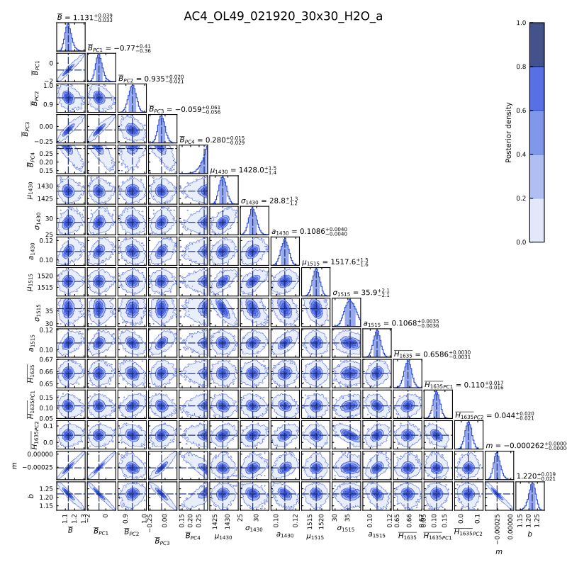
The pairwise figure plots the posterior probability density distribution for the 16 fitting parameters of Equation 10, allowing for the visualization of covariance within the parameters. Accounting for covariance allows us to properly account for uncertainty.
[15]:
Image("https://github.com/sarahshi/PyIRoGlass/raw/main/docs/_static/AC4_OL49_021920_30x30_H2O_a_pairwise.png")
[15]:
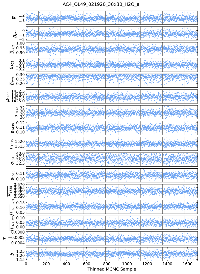
The trace figure shows how the parameters evolve through MCMC sampling.
[16]:
Image("https://github.com/sarahshi/PyIRoGlass/raw/main/docs/_static/AC4_OL49_021920_30x30_H2O_a_trace.png")
[16]:
LOG and NPZ
.log files record the performance of the MCMC algorithm through the samples, and the best parameters at each 10% increment. These are shown above.
.npz files store all the best-parameters, sampled parameters, etc. in a ready-to-use NumPy format.
We won’t open these here, but these are quite useful to review!
Concentrations
We now want to convert all those peak heights (with uncertainties) to concentrations (with uncertainties), by applying the Beer-Lambert Law. We do so by using the pig.calculate_concentrations function, which takes in these parameters and samples over N samples for a secondary MCMC:
Volatile_PH: DataFrame with peak heights and their associated uncertainties; the output frompig.calculate_baselineschemistry: DataFrame of chemical datathickness: DataFrame of thickness dataexport_path: Output directory name, orNoneto prevent figure generationN: Number of Monte Carlo simulations to perform for uncertainty estimation, with default of 500,000T: Temperature in Celsius at which the density is calculated, with default of 25°CP: Pressure in bars at which the density is calculated, with default of 1 barmodel: Choice of density model, with options of the default “LS” for Lesher and Spera (2015) and “IT” for Iacovino and Till (2019)
[17]:
concentrations_df = pig.calculate_concentrations(Volatile_PH, chemistry, thickness, export_path)
We’re all done now! Let’s display the concentrations_df DataFrame, which contains all results.
[18]:
concentrations_df
[18]:
| H2Ot_MEAN | H2Ot_STD | H2Ot_3550_M | H2Ot_3550_STD | H2Ot_3550_SAT | H2Om_1635_BP | H2Om_1635_STD | CO2_MEAN | CO2_STD | CO2_1515_BP | ... | epsilon_H2Ot_3550 | sigma_epsilon_H2Ot_3550 | epsilon_H2Om_1635 | sigma_epsilon_H2Om_1635 | epsilon_CO2 | sigma_epsilon_CO2 | epsilon_H2Om_5200 | sigma_epsilon_H2Om_5200 | epsilon_OH_4500 | sigma_epsilon_OH_4500 | |
|---|---|---|---|---|---|---|---|---|---|---|---|---|---|---|---|---|---|---|---|---|---|
| AC4_OL49_021920_30x30_H2O_a | 2.548444 | 0.161081 | 2.420676 | 0.189704 | * | 1.301475 | 0.190134 | 754.152544 | 36.582302 | 745.935232 | ... | 66.142594 | 7.503769 | 37.322108 | 8.645060 | 258.429949 | 18.362798 | 1.009458 | 0.300803 | 0.861196 | 0.279571 |
| AC4_OL53_101220_256s_30x30_a | 4.036919 | 0.432274 | 4.036919 | 0.432274 | - | 1.49134 | 0.258304 | 737.553149 | 62.248309 | 756.185932 | ... | 64.493655 | 7.380834 | 34.452486 | 8.504269 | 293.261300 | 16.287120 | 0.901474 | 0.295829 | 0.779611 | 0.274924 |
| STD_D1010_012821_256s_100x100_a | 0.901034 | 0.096678 | 1.201368 | 0.087904 | * | 0.153231 | 0.025398 | 156.607591 | 7.265153 | 165.48701 | ... | 62.751984 | 7.251813 | 31.421482 | 8.354348 | 311.700491 | 15.127604 | 0.787418 | 0.290510 | 0.693438 | 0.270004 |
3 rows × 35 columns
There are a few things to note. Each column with the suffix _MEAN represents the mean value, _BP represents the best-parameter from MCMC, and _STD represents the standard deviation. We recommend the use of the H2Ot_MEAN, H2Ot_STD, CO2_MEAN, and CO2_STD columns. The columns with the suffix _STN show the signal-to-noise ratio of the NIR peaks, and the columns with the prefix ERR_ just process this information, returning a - if the peaks are meaningful and a
* if the signal is too low.
Concentrations of \(\mathrm{H_2O}\) depend on whether your sample is saturated or not. If your sample is unsaturated (marked by H2Ot_3550_SAT=='-'), the column H2Ot_MEAN==H2Ot_3550_M. If your sample is saturated (marked by H2Ot_3550_SAT=='*'), the column of H2Ot_MEAN==(H2Om_1635_BP+OH_4500_M). The \(\mathrm{H_2O_{t, 3550}}\) peak cannot be used, given potential nonlinearity in the Beer-Lambert Law. See the discussion of this handling of speciation in the paper.
The column Density contains the densities used for the final concentration. The values between Density and Density_Sat will be different if the sample is saturated, showing the difference in densities when using variable concentrations of \(\mathrm{H_2O_m}\).
Tau and Eta calculate the compositional parameters required for determining molar absorptivity. All calculated molar absorptivities and their uncertainties (Sigma_ prefix) from the inversion are provided in the DataFrame.